Steve: A model for supernova cosmology

As surveys discover greater numbers of supernova, our analyses become limited by systematics rather than data. Hierarchical Bayesian models are perfect for incorporating subtle effects into our model, and so I made one to do just that.

Supernova cosmology works because Type Ia supernova represent standardisable candles. That is, with a few factors taken into account, they are essentially all the same brightness. Which means, if we see two supernovae, and one is four times dimmer than the other, it must be twice as far away. So we have (relative) distance. And we can measure the redshift of the event, which is a measure of how much the expansion of the universe has stretched the light from the supernovae. And by combining those two measurements, we can ask questions like “How much dark matter is there in the universe?”

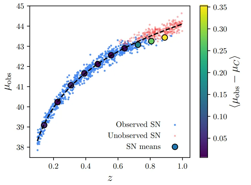
One of the main challenges with supernova cosmology is to correct for something called Malmquist bias. Supernova aren’t perfect standard candles, some are a bit brighter and bluer, some are dimmer and redder. But our analyses depend on being able to measure the population itself.

However, when supernova are far away and so dim we can barely detect them, well, we’re only going to see the brighter ones. The dimmer ones will be to faint for our telescopes. Take a look at the figure below, which has redshift on the x-axis and distance on the y-axis. If we try and find the average brightness as a function of redshift we start getting biases once we start missing supernovae.


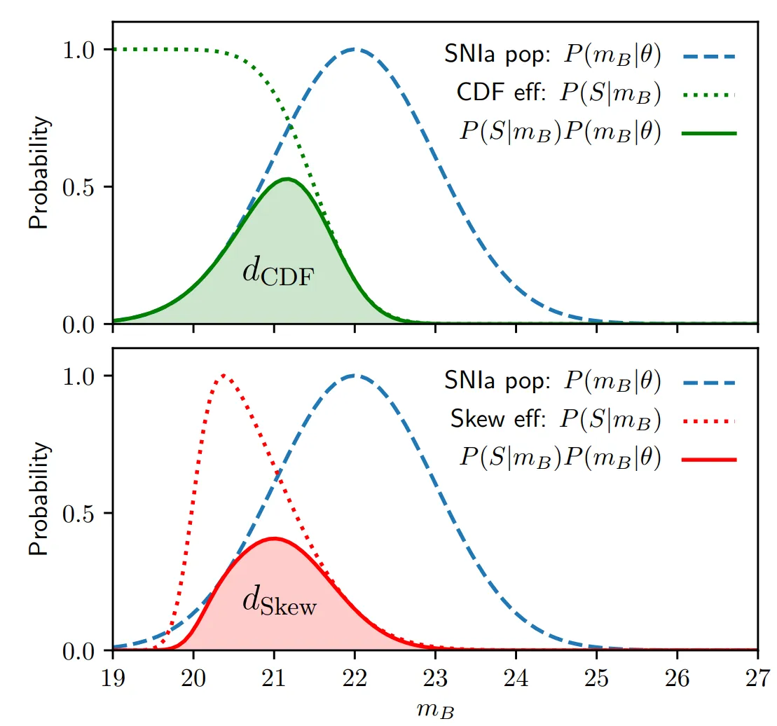
The way many analyses correct for this is to calculate how much we expect to get the answer wrong by and then correct the data by this amount. Instead of doing this, I’ve incoporated Malmquist bias directly inside my model, so it becomes a prediction instead of something to correct for. I do this essentially by some nasty integrals, designed to compute the probability that we’d observe a supernova given a redshift. The integral is given by the area under the curve in the plot below.

Of course, this is only a small part of the model. The other parameters and their conditional probabilities are described in the PGM below. Don’t get fixated on the diagram unless you want to read the paper here.


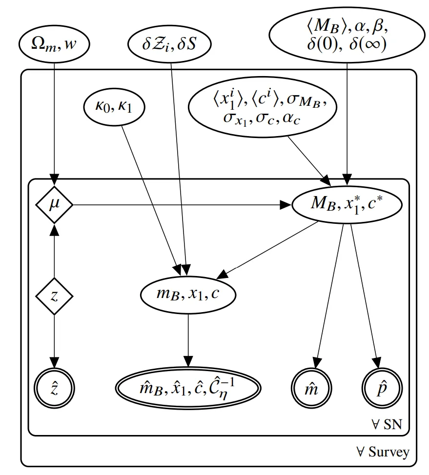
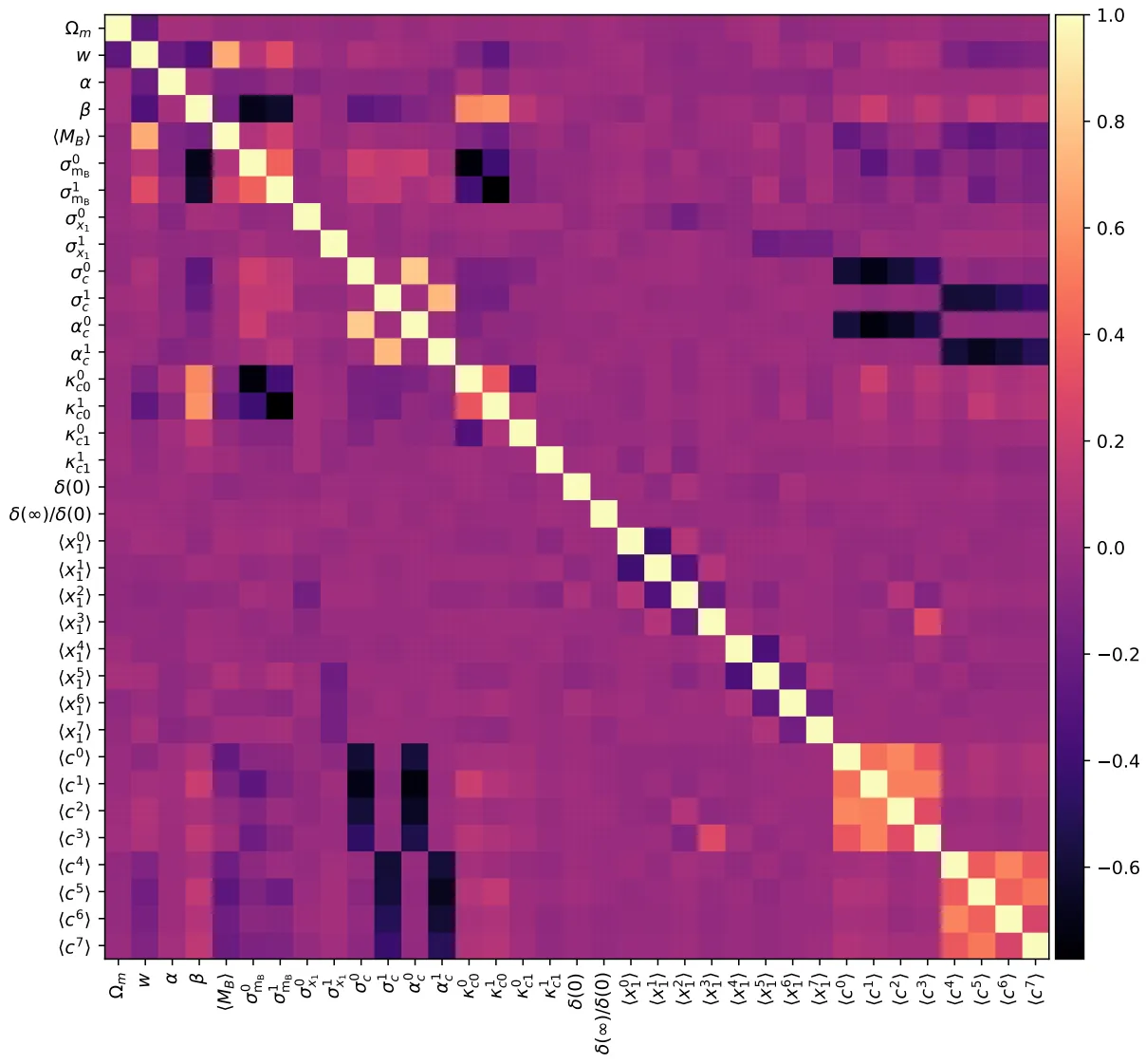
Actually, the number of parameters in this model makes it incredible difficult to fit. Each supernova has two parameters, plus everything else. For a few hundred supernova, we’re almost at a thousand parameters. And searching that many dimensions to find the best fitting value is actually a real pain. Especially with so many of the parameters highly correlated. The correlation plot shows just some of the top level parameters. Ideally, I’d want it to be completely diagonal, all the bright and dark squares are correlated and anti-correlated parameters, making my life more difficult!

![](corr.jpg" class=" img-invert)

Thankfully, we utilised Stan and the joy of Hamiltonian Monte-Carlo to sample the parameter space in finite time, getting the familiar banana-shaped cosmology contour you can see below.

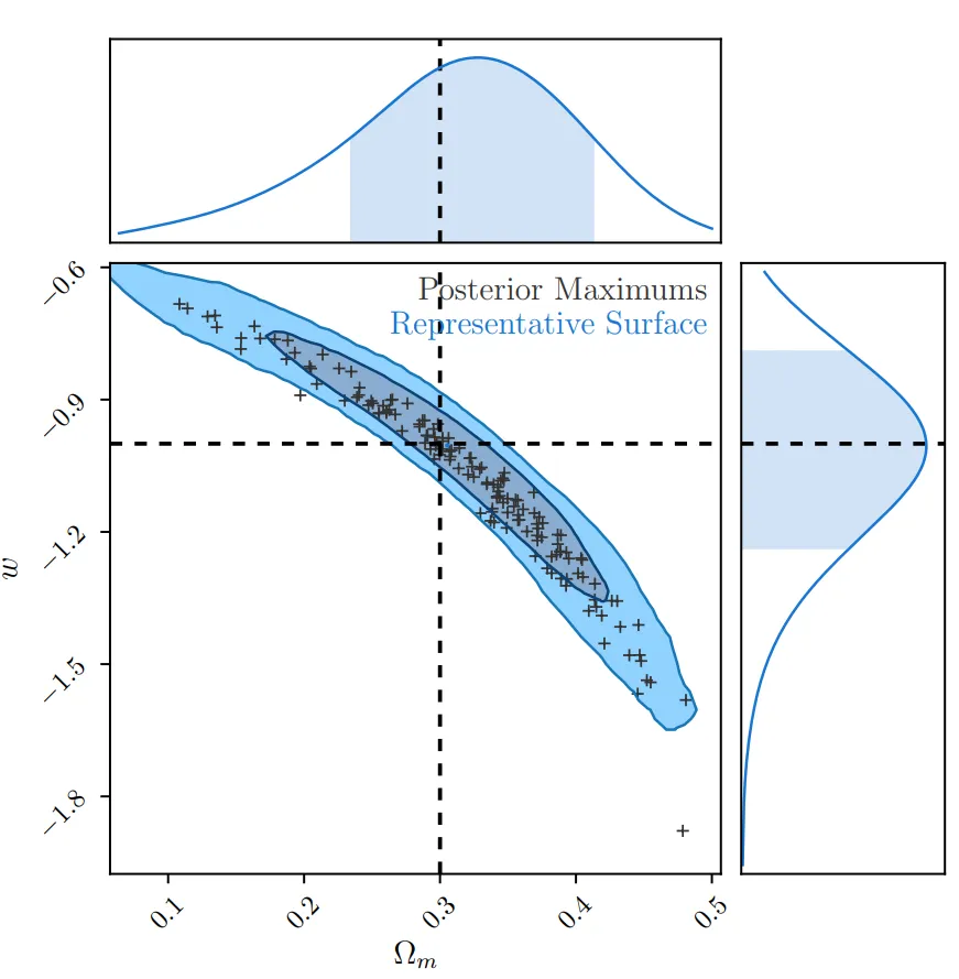
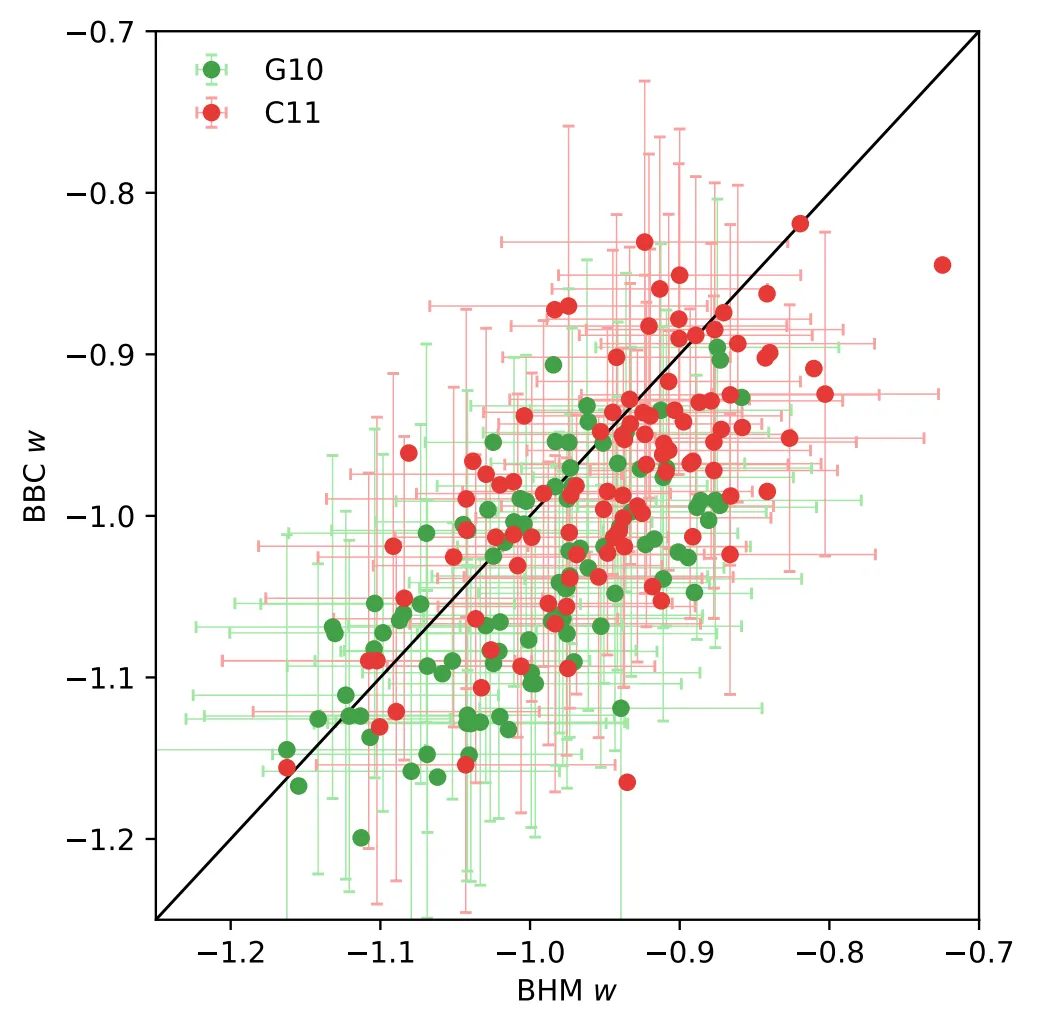
Of interest, because it implies future work, is a systematic difference between my method (BHM) and a method which corrects the data (BBC). Turns out we still don’t understand the dispersion of the supernova population well enough, so we’ll have to work on that if we want to get better constraints on dark energy and dark matter.

![](bbc_vs_bhm.jpg" class=" img-invert)