Bayesian Linear Regression in Python
2019-07-27
A tutorial from creating data to plotting confidence intervals.
Bayesian linear regression is a common topic, but allow me to put my own spin on it. We’ll start at generating some data, defining a model, fitting it and plotting the results. It shouldn’t take long.
Generating Data
Let’s start by generating some experimental data. For simplicity, let us assume some underlying process generates samples and our observations have some given Gaussian error .
import matplotlib.pyplot as plt
import numpy as np

rng = np.random.default_rng(0)
num_points = 20
m, c = np.tan(np.pi / 4), -1  # So our angle is 45 degrees, m = 1
xs = rng.uniform(size=num_points) * 10 + 2
ys = m * xs + c
err = np.sqrt(ys)
ys += err * rng.normal(size=num_points)
Now, let’s plot our generated data to make sure it all looks good.
fig, ax = plt.subplots(figsize=(8, 3))
ax.errorbar(xs, ys, yerr=err, fmt=".", label="Observations", ms=5)
ax.legend(frameon=False, loc=2)
ax.set_xlabel("x")
ax.set_ylabel("y");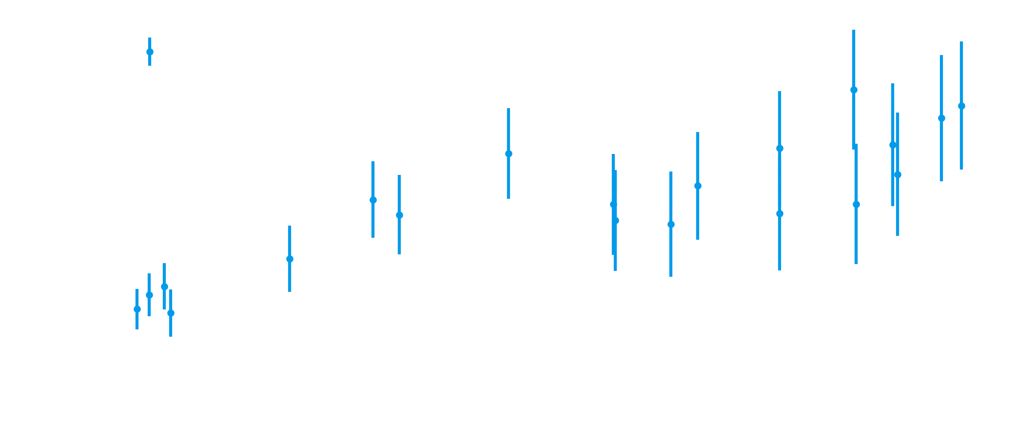
And it does. Notice that in this data, the further you are along the x-axis, the more uncertainty we have.
Defining a model
So, let’s recall Bayes’ theorem for a second:
where is our model parametrisation and is our data. To sub in nomenclature, our posterior is proportional to our likelihood multiplied by our prior. So, we need to come up with a model to describe data, which one would think is fairly straightforward, given we just coded a model to generate our data. But before we jump the gun and code up , let us also consider the model .
Why would we care about whether we use a gradient or an angle? Well, it comes down to simplifying our prior - in our case with no background knowledge we’d want to sample all of our parameter space with the same probability. But what happens if we plot uniform probability in the two separate models?
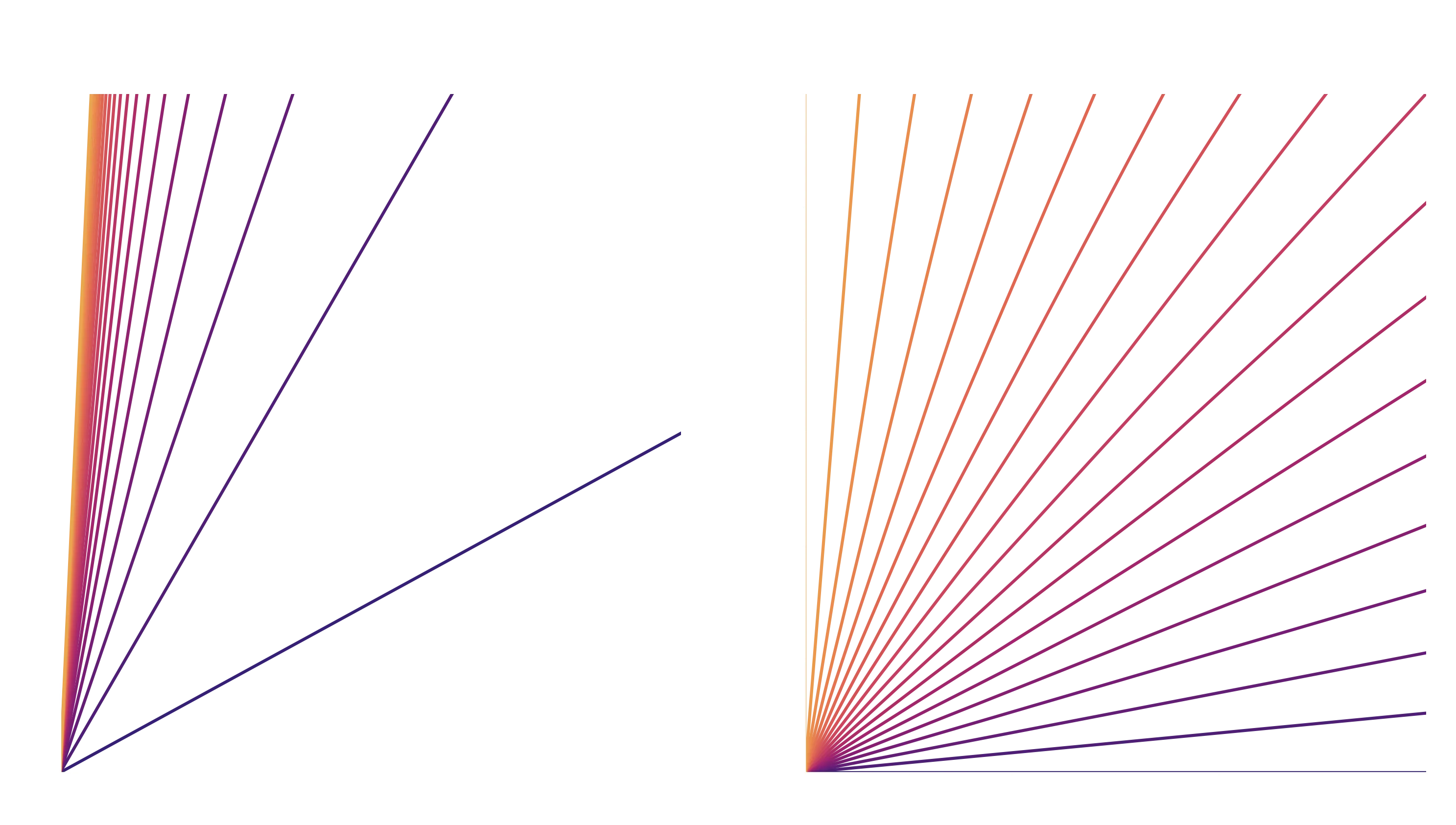
Now it seems to me that uniformly sampling the angle, rather than the gradient, gives us an even distribution of coverage over our observational space.
So, if we lock in that model, we have two parameters of interest: . Next up, we should think about the priors on those two parameters. Luckily, with the little investigation we did before, we can comfortably set flat (uniform) priors on both and and they will be non-informative. Aka, they will not contribute at all to our fitting locations. Note that we could have pursued the model parametrised by gradient, and simply given a non-uniform prior, but this way is easier. More formally, we have that:
Where yes, we’re working in radians. In code, this is also as simple:
def log_prior(xs) -> float:
    phi, c = xs
    if np.abs(phi) > np.pi / 2:
        return -np.inf
    return 0
Notice we don’t even care about at all in the code, it can be any value, and the prior is constant over that value. And because Bayes’ theorem only cares about proportionality, if it doesn’t change, we don’t worry about it. We only care about ‘s boundary conditions for the same reasons, and when it crosses the boundary to a location we say it can’t go, we return , which - as this is the log prior, is the same as saying probability zero. It can’t happen.
As a note, we always work in log probability space, not probability space, because the numbers tend to span vast orders of magnitude.
Now we have the likelihood function to think about. If we take the errors as normally distributed (which we know they are), we can write down
where is the unit normal. This makes the assumption our observations are independent, which holds for this case. Note here that the equation is for a single data point. For a dataset, we would want this for each point:
When working in log space, this product simply becomes a sum. Writing out this equation is normally the hard part, implementing it in code is simple:
from scipy.stats import norm


def log_likelihood(xs, data) -> float:
    phi, c = xs
    xobs, yobs, eobs = data
    model = np.tan(phi) * xobs + c
    diff = model - yobs
    return norm.logpdf(diff / eobs).sum()
And now we want a function that gets the log posterior, by combining the prior and likelihood. Notice that if the prior comes back as an impossible value, we won’t waste time computing the likelihood, we’ll just return straight away.
def log_posterior(xs, data) -> float:
    prior = log_prior(xs)
    if not np.isfinite(prior):
        return prior
    return prior + log_likelihood(xs, data)
With that, our model is fully defined. We can now try and fit it to the data to see how we go.
Model Fitting
There are so many ways of doing this. Using some MCMC algorithm, using nested sampling, other algorithms… too many options. Initially I wanted to do this example using dynesty - a new nested sampling package for python. But I realised, better to start off with the simpler emcee implementation to begin with. emcee is an affine-invariant MCMC sampler, and if you want more detail on that, check out its documentation, let’s just jump into how you’d use it.
So let’s break this down. ndim is the number of parameters we have to fit, and we want to make sure that we have multiple times this for our nwalkers value, where each walker is a tracked position in parameter space that gets explored in a probabilistic fashion. I usually make sure there are a minimum of thirty or so walkers, but the more the merrier.
Next up, p0 - each walker in the process needs to start somewhere! In this case, we pick a random position, it’ll move from this quickly. We then make the sampler, and tell each walker in the sampler to take 8000 steps. The walkers should move around the parameter space in a way thats informed by the posterior (given our data). Now, the initial phase where the walkers move from the random positions we set to exploring the space properly is known as burn in, and we want to get rid of it, so we throw out the first 200 of the 8000 steps. How many you throw out depends on your problem, see the emcee documentation for more discussion on this, or just keep reading. Finally, we take the 3D chain (num walkers x num steps x num dimensions) and squish it down to 2D.
Interpreting chains
So, we have this sampler, and it will have taken, you guessed it, samples of the posterior surface. How do we use this?
The important thing to know is that an MCMC samples areas in parameter space proportional to their probability. So a point in space which is twice as likely as another will have twice as many samples. There are libraries you can use where you throw in those samples and it will crunch the numbers for you and give you constraints on your parameters. We’ll be using one I made, called ChainConsumer.
If you don’t want to use an external library, you can get the array of samples using sampler.get_chain(flat=True), but why make life harder than it needs to be. We’ll throw out the first 200 points as burn in and check to see if everything is mixed nicely.

So here we can see the walks plotted, also known as a trace plot. The blue contains all the samples from the chain we removed the burn in from. If you notice little ticks or spikes in your trace plot, you probably need to discard more initial points to allow the chains to burn in properly. What we want to do here is check that the chains are stationary (not meandering around), and we can’t tell what’s in one walker to another (ie imagine if you took all the points from 20k to 40k and shifted them all up, that would be a stuck walker). The fact we don’t see this in the blue means we’ve probably removed all burn in and we’re getting good samples.
There are diagnostics to check this in ChainConsumer too, but its not needed for this simple example.
Up next - let’s get actual parameter constraints from this!
c.plotter.plot()
summary = c.analysis.get_summary()["emcee"]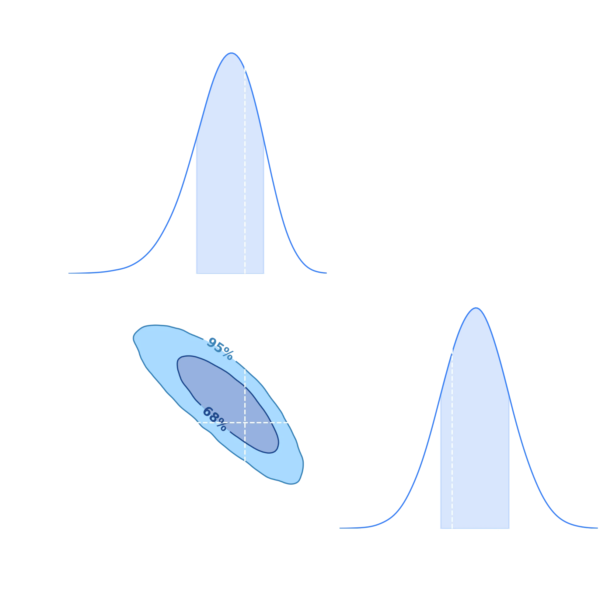
So how do we read this? Well, if you look at the summary printed, that gives the bounds for the lower uncertainty, maximum value, and upper uncertainty respectively (uncertainty being the 68% confidence levels). In the actual plot, you can see a 2D surface which represents our posterior. For example, the inner circle, labelled 68%, says that 68% of the time the true value for and will lie in that contour. 95% of the time it will lie in the broader contour.
Finally, one thing we might want to do is to plot the best fitting model and its uncertainty against our data. The best fit part is easy, its the uncertainty on our model that is the trickier part. What we’ll do is sample from our chain over a variety of x-values to determine the effect our parameter uncertainty has in observational space. Easier to do than explain.
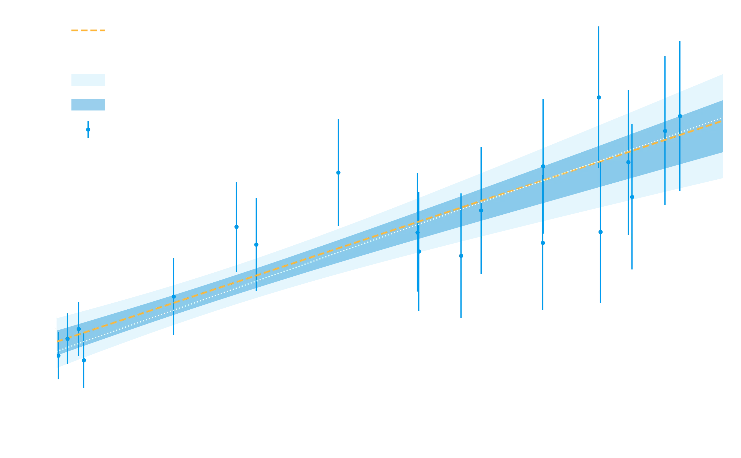
Notice how even with a linear model, our uncertainty is not just linear, it is smallest in the center of the dataset, as we might expect if we imagine the fit rocking the line like a see-saw during the fitting process. To reiterate, what we did to calculate the uncertainty was - instead of using some summary of the uncertainty like the standard deviation - we used the entire posterior surface to generate thousands of models, and looked at their uncertainty (using the percentile) function to get the and bounds (the norm.cdf part) to display on the plot. For more examples on this methd of propagating uncertainty, see here.
And that’s it, those are the basics.
- Define your model, think about parametrisation, priors and likelihoods
- Create a sampler and sample your parameter space
- Determine parameter constraints from your samples.
- Plot everything.
For your convenience, here’s the code in one block:
import matplotlib.pyplot as plt
import numpy as np
rng = np.random.default_rng(0)
num_points = 20
m, c = np.tan(np.pi / 4), -1 # So our angle is 45 degrees, m = 1
xs = rng.uniform(size=num_points) * 10 + 2
ys = m * xs + c
err = np.sqrt(ys)
ys += err * rng.normal(size=num_points)
fig, ax = plt.subplots(figsize=(8, 3))
ax.errorbar(xs, ys, yerr=err, fmt=".", label="Observations", ms=5)
ax.legend(frameon=False, loc=2)
ax.set_xlabel("x")
ax.set_ylabel("y");
def log_prior(xs) -> float:
phi, c = xs
if np.abs(phi) > np.pi / 2:
return -np.inf
return 0
from scipy.stats import norm
def log_likelihood(xs, data) -> float:
phi, c = xs
xobs, yobs, eobs = data
model = np.tan(phi) * xobs + c
diff = model - yobs
return norm.logpdf(diff / eobs).sum()
def log_posterior(xs, data) -> float:
prior = log_prior(xs)
if not np.isfinite(prior):
return prior
return prior + log_likelihood(xs, data)
import emcee

ndim = 2  # How many parameters we are fitting. This is our dimensionality.
nwalkers = 50  # Keep this well above your dimensionality.
p0 = rng.uniform(low=-1.5, high=1.5, size=(nwalkers, ndim))  # Start points
sampler = emcee.EnsembleSampler(nwalkers, ndim, log_posterior, args=[(xs, ys, err)])
sampler.run_mcmc(p0, 8000);  # Tell each walker to take 8000 steps
from chainconsumer import Chain, ChainConsumer, PlotConfig, Truth

chain = Chain.from_emcee(
    sampler,
    columns=["phi", "c"],  # Names of our parameters
    name="emcee",
    discard=200,  # Removes our burn-in
    show_contour_labels=True,  # Used in plotting
)
truth = Truth(location={"c": -1, r"phi": np.pi / 4}, color="white")
c = ChainConsumer()
c.add_chain(chain)
c.add_truth(truth)
c.set_plot_config(PlotConfig(labels={"phi": "$\\phi$", "c": "$c$"}))  # To get nice labels
c.plotter.plot_walks(figsize=(8, 4));
c.plotter.plot()
summary = c.analysis.get_summary()["emcee"]
x_vals = np.linspace(2, 12, 30)
# Calculate best fit
phi_best = summary["phi"].center
c_best = summary["c"].center
best_fit = np.tan(phi_best) * x_vals + c_best

gradients = np.tan(chain.samples["phi"].to_numpy())
offsets = chain.samples["c"].to_numpy()

# For each x_value, we want to get all the realisations of y
# Its easiest to do this via matrix multiplication
realisations = gradients[:, None] * x_vals[None, :] + offsets[:, None]
# So now realisations will be a 2D array, one row for each sample, one column for each x value
# Which makes it easy to take the CDF at each X value
bounds = np.quantile(realisations, norm.cdf([-2, -1, 1, 2]), axis=0)

# Plot everything
fig, ax = plt.subplots(figsize=(10, 6))
ax.errorbar(xs, ys, yerr=err, fmt=".", label="Observations", ms=5, lw=1)
ax.plot(x_vals, best_fit, label="Best Fit", c="#ffb638")
ax.plot(x_vals, x_vals - 1, label="Truth", c="w", ls=":", lw=1)
plt.fill_between(x_vals, bounds[0, :], bounds[-1, :], label="95\% uncertainty", fc="#03A9F4", alpha=0.1)
plt.fill_between(x_vals, bounds[1, :], bounds[-2, :], label="68\% uncertainty", fc="#0288D1", alpha=0.4)
ax.legend(frameon=False, loc=2)
ax.set_xlabel("x"), ax.set_ylabel("y"), ax.set_xlim(2, 12);